Create basic XY scatter plot for quick data exploration. Default to show Pearson correlation coefficient with p-value using ggpubr::stat_cor. For more complex plots, it is recommended to use ggplot2::ggplot2 directly.
Usage
ggxy(
  d,
  x,
  y,
  ...,
  lm = TRUE,
  se = TRUE,
  cor = TRUE,
  pv = NULL,
  nsub = TRUE,
  legend = TRUE,
  asp = 1
)
Arguments
- d
<dfr>A data frame.- x, y
<var>Variables for x- and y-axis as unquoted names.- ...
Arguments to pass to ggplot2::aes for additional mapping.
- lm
<lgl>TRUEto add regression line from linear model.- se
<lgl>TRUEto show standard error with the regression line.- cor
<lgl>TRUEto show Pearson correlation coefficient with p-value.- pv
<dbl>Precision for the p-value, e.g., 0.001 to show 3 decimal places.- nsub
<lgl>Show number of observations.- legend
<lgl>TRUEto show legend.- asp
<num>Foraspect.ratioin ggplot2::theme.
Examples
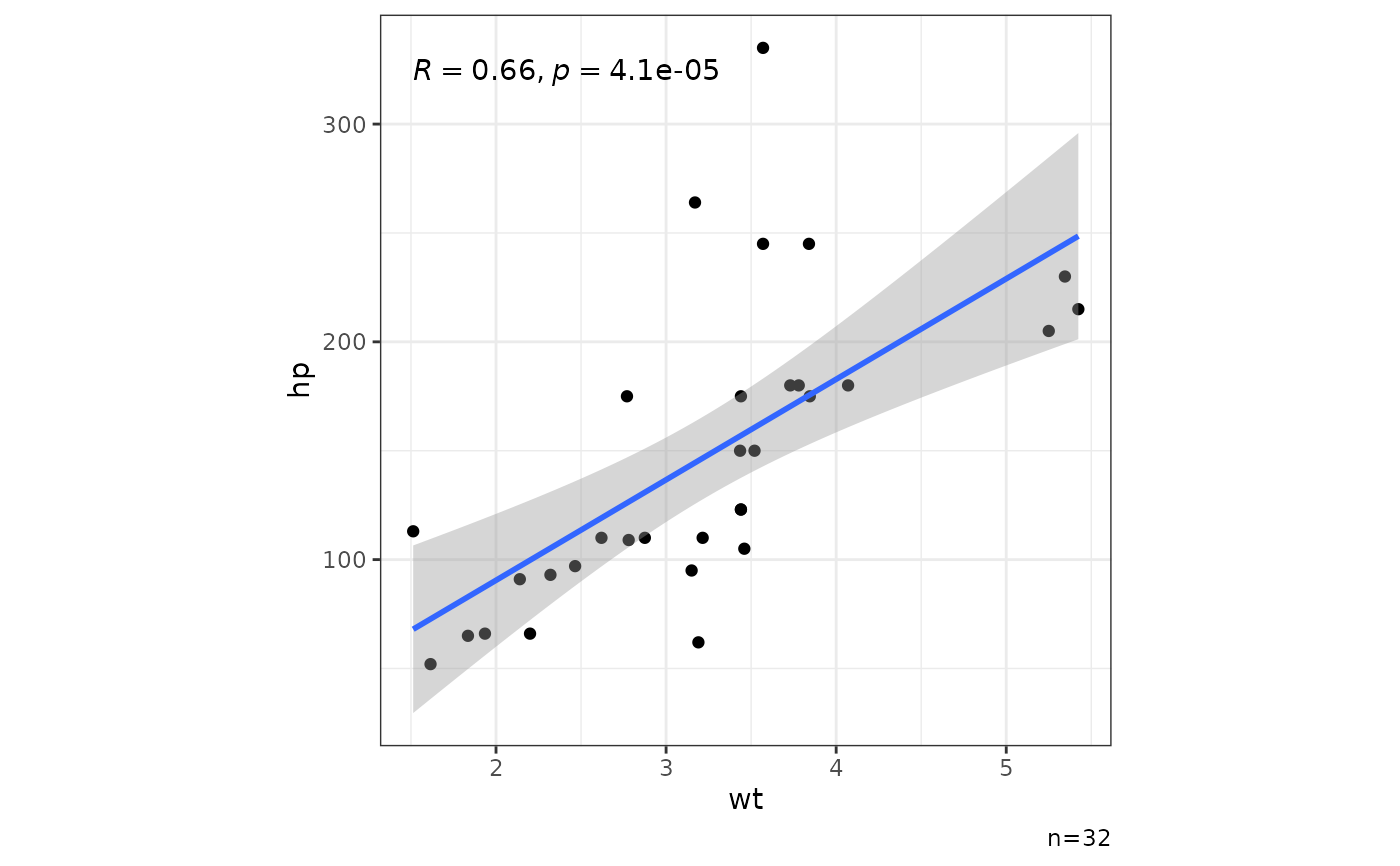
mtcars |> ggxy(wt,hp)
#> `geom_smooth()` using formula = 'y ~ x'
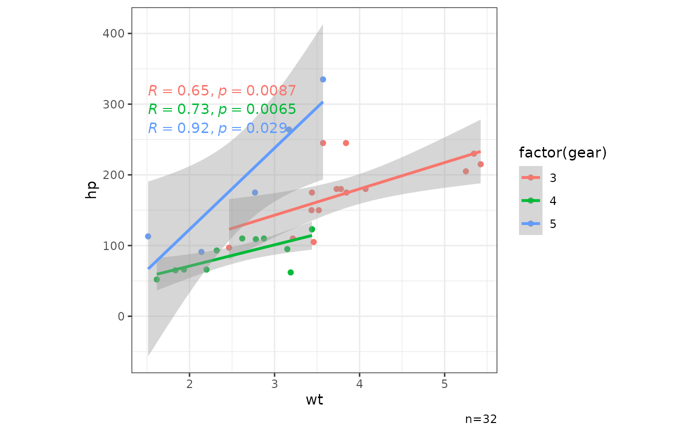
 mtcars |> ggxy(wt,hp,col=factor(gear))
#> `geom_smooth()` using formula = 'y ~ x'
mtcars |> ggxy(wt,hp,col=factor(gear))
#> `geom_smooth()` using formula = 'y ~ x'
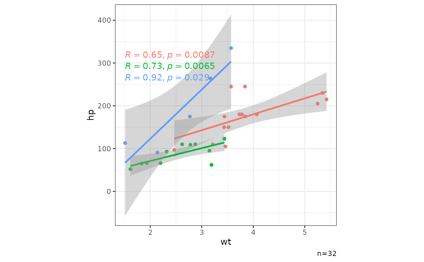
 mtcars |> ggxy(wt,hp,col=factor(gear),legend=FALSE)
#> `geom_smooth()` using formula = 'y ~ x'
mtcars |> ggxy(wt,hp,col=factor(gear),legend=FALSE)
#> `geom_smooth()` using formula = 'y ~ x'
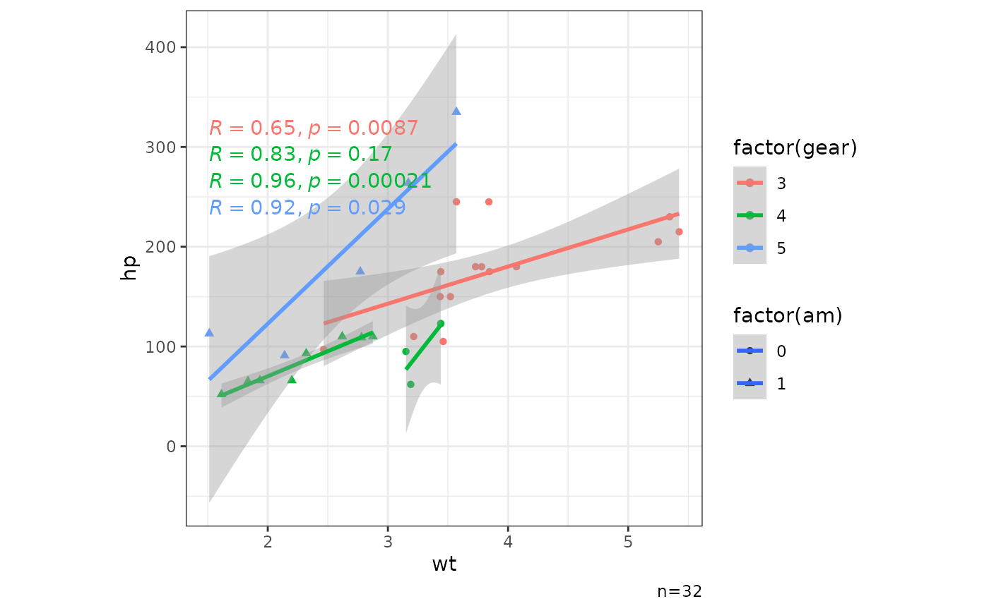
 mtcars |> ggxy(wt,hp,col=factor(gear),pch=factor(am))
#> `geom_smooth()` using formula = 'y ~ x'
mtcars |> ggxy(wt,hp,col=factor(gear),pch=factor(am))
#> `geom_smooth()` using formula = 'y ~ x'
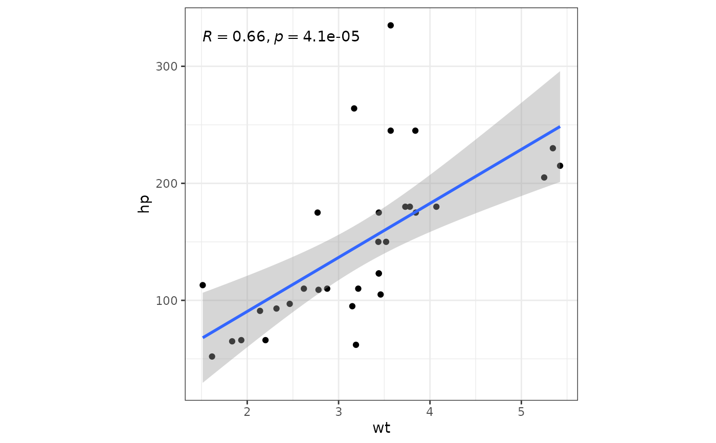
 mtcars |> ggxy(wt,hp,nsub=FALSE)
#> `geom_smooth()` using formula = 'y ~ x'
mtcars |> ggxy(wt,hp,nsub=FALSE)
#> `geom_smooth()` using formula = 'y ~ x'
 mtcars |> ggxy(wt,hp,pv=0.001)
#> `geom_smooth()` using formula = 'y ~ x'
mtcars |> ggxy(wt,hp,pv=0.001)
#> `geom_smooth()` using formula = 'y ~ x'
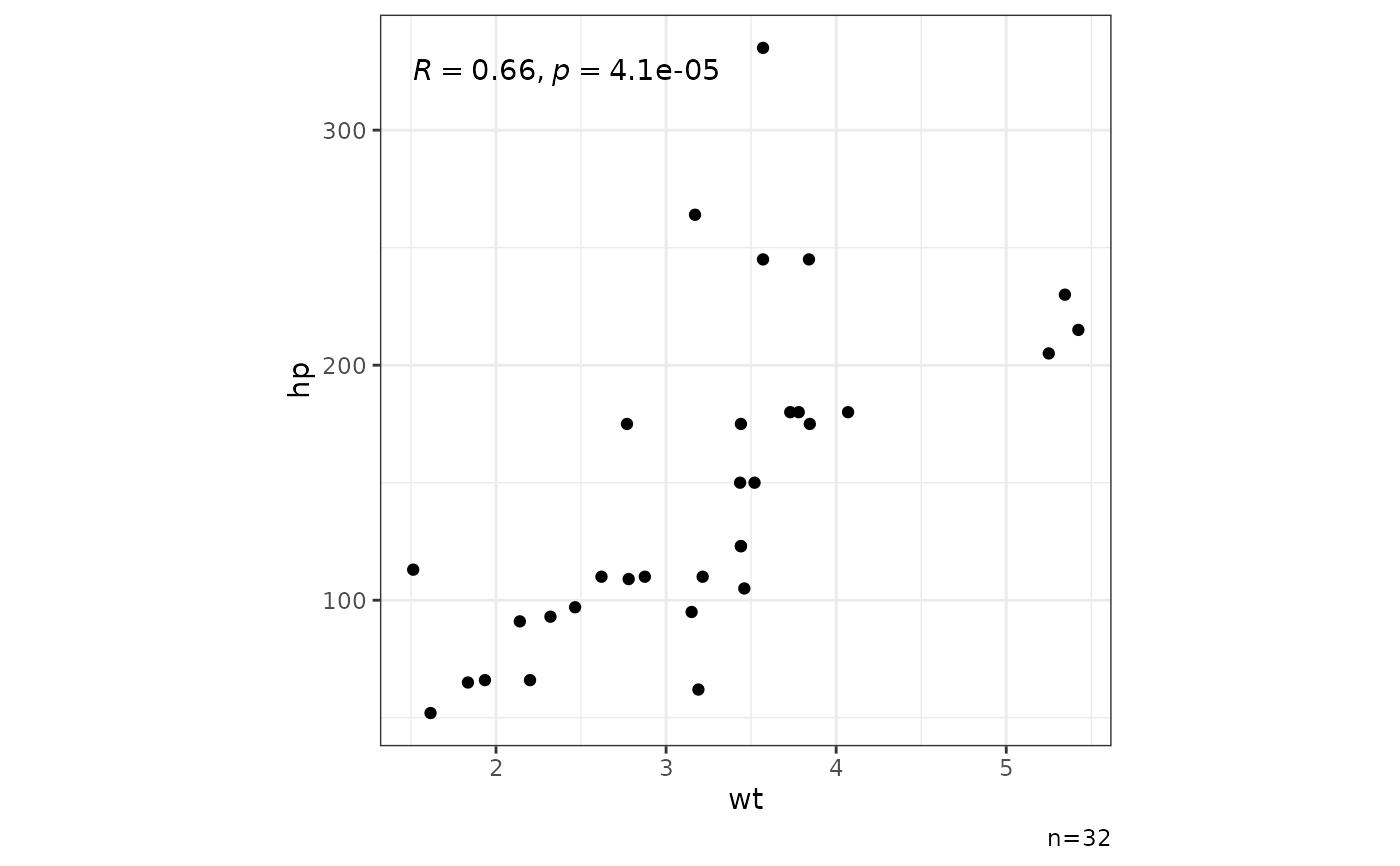
 mtcars |> ggxy(wt,hp,lm=FALSE)
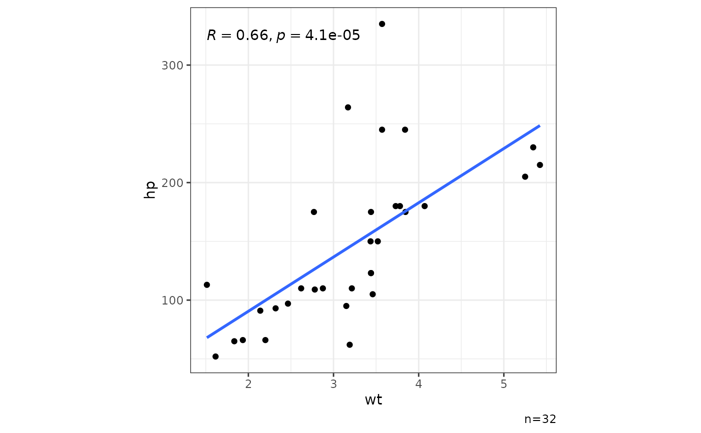
 mtcars |> ggxy(wt,hp,se=FALSE)
#> `geom_smooth()` using formula = 'y ~ x'
mtcars |> ggxy(wt,hp,se=FALSE)
#> `geom_smooth()` using formula = 'y ~ x'
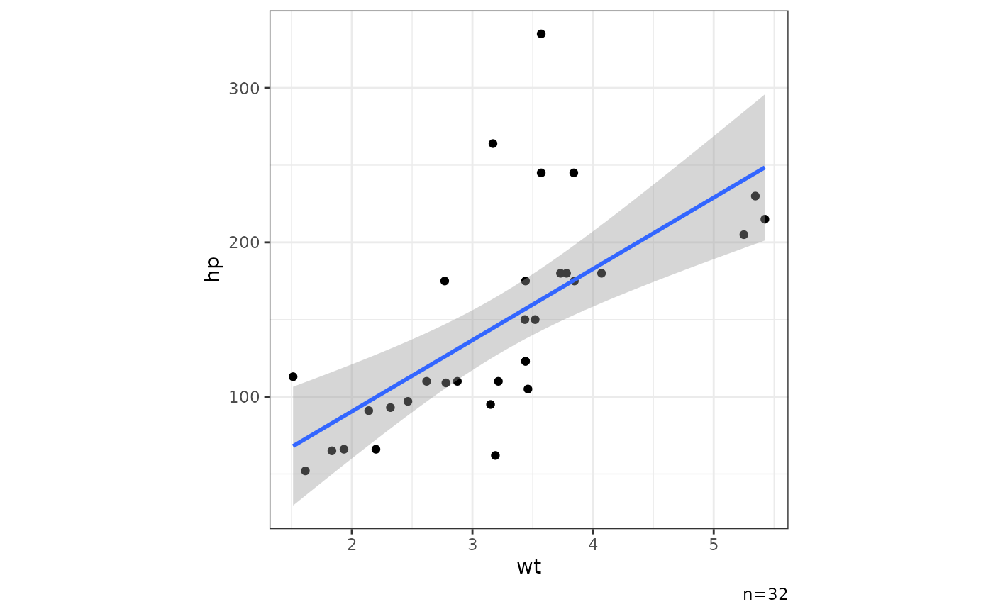
 mtcars |> ggxy(wt,hp,cor=FALSE)
#> `geom_smooth()` using formula = 'y ~ x'
mtcars |> ggxy(wt,hp,cor=FALSE)
#> `geom_smooth()` using formula = 'y ~ x'